Digital Image Processing using OpenCV

Updated: Aug 5, 2021

OpenCV (Open Source Computer Vision Library) is an open source computer vision and machine learning software library. It is used to detect and recognize faces, identify objects, classify human actions in videos, track camera movements, track moving objects, extract 3D models of objects, produce 3D point clouds from stereo cameras, etc. In this blog, we will discuss about the various methods of image processing using OpenCV, it’s application and it’s benefits.

Before we start, Let's download the OpenCV package

pip install opencv-python

The very first step is Thresholding

It is one of the most common segmentation techniques in computer vision and it allows us to separate the foreground (i.e., the objects that we are interested in) from the background of the image.

Thresholding comes in two forms:

We have simple thresholding where we manually supply parameters to segment the image — this works extremely well in controlled lighting conditions where we can ensure high contrast between the foreground and background of the image.
Next we have adaptive thresholding which, instead of trying to threshold an image globally using a single value, instead breaks the image down into smaller pieces, and thresholds each of these pieces separately and individually.

import cv2 as cv
import numpy as np
from matplotlib import pyplot as plt
 # read an image in grayscale
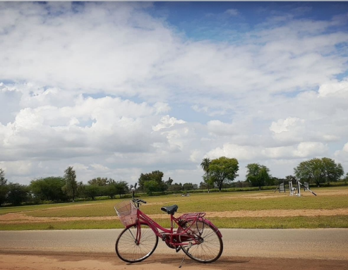
img = cv.imread('C:/images/cycle.jpg',0)
img = cv.resize(img, (320,225))
 # apply various thresholds
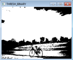
val, th1 = cv.threshold(img, 110, 255, cv.THRESH_BINARY)
val, th2 = cv.threshold(img, 110, 255, cv.THRESH_BINARY_INV)
val, th3 = cv.threshold(img, 110, 255, cv.THRESH_TRUNC)
val, th4 = cv.threshold(img, 110, 255, cv.THRESH_TOZERO)
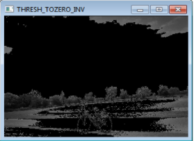
val, th5 = cv.threshold(img, 110, 255, cv.THRESH_TOZERO_INV)
 # display the images
cv.imshow('Original', img)
cv.imshow('THRESH_BINARY', th1)
cv.imshow('THRESH_BINARY_INV', th2)
cv.imshow('THRESH_TRUNC', th3)
cv.imshow('THRESH_TOZERO', th4)
cv.imshow('THRESH_TOZERO_INV', th5)
cv.waitKey(0)
cv.destroyAllWindows()

Some of the outputs are:

We can also implement adaptive thresholding:

import cv2 as cv
import numpy as np
from matplotlib import pyplot as plt
img = cv.imread('C:/images/cycle.jpg', 0)
img = cv.resize(img, (320,225))
 # apply various adaptive thresholds
th1=cv.adaptiveThreshold(img,255,cv.ADAPTIVE_THRESH_MEAN_C,cv.THRESH_BINARY, 7, 4)
th2=cv.adaptiveThreshold(img,255,cv.ADAPTIVE_THRESH_GAUSSIAN_C,cv.THRESH_BINARY, 7, 4)

Image smoothing

Image smoothing is an important image processing technique that performs blurring and noise filtering in an image. It finds applications in preprocessing and postprocessing of deep learning models. In general, smoothing is performed by a 2D kernel of a specific size on each channel of the image. The kernel average of neighborhoods yields the resulting image. It is of 4 types:

Simple average blurring
Gaussian blurring
Median filtering
Bilateral filtering

Simple average blurring:- it takes an area of pixels surrounding a central pixel, averages all these pixels together, and replaces the central pixel with the average. By taking the average of the region surrounding a pixel, we are smoothing it and replacing it with the value of its local neighborhood. This allows us to reduce noise and the level of detail, simply by relying on the average.

import cv2 as cv
import numpy as np
from matplotlib import pyplot as plt
img = cv.imread('C:/images/cycle.jpg', 1)
img = cv.resize(img, (300,300))
 # Apply blur
img1 = cv.blur(img,(3,3))
 # display the images
cv.imshow('Original', img)
cv.imshow('Blur', img1)
cv.waitKey(0)
cv.destroyAllWindows()

After Blur

Original image

Gaussian blurring:- It is similar to average blurring, but instead of using a simple mean, we are now using a weighted mean, where neighborhood pixels that are closer to the central pixel contribute more “weight” to the average.

import cv2 as cv
import numpy as np
from matplotlib import pyplot as plt
img = cv.imread('C:/images/cycle.jpg', 1)
img = cv.resize(img, (320,210))
 # Apply Gaussian blur
img1 = cv.GaussianBlur(img,(5,5),2)
 # display the images
cv.imshow('Original', img)
cv.imshow('Gaussian', img1)
cv.waitKey(0)
cv.destroyAllWindows()

Median blur:- it is known for its salt-and-pepper noise removal. Unwanted small white and black dots on an image are removed with this tool.

import cv2 as cv
import numpy as np
from matplotlib import pyplot as plt
img = cv.imread('C:/images/cycle.jpg', 0)
img = cv.resize(img, (320,210))
 # Apply median blur
img1 = cv.medianBlur(img,3)
 # display the images
cv.imshow('Original', img)
cv.imshow('Median', img1)
cv.waitKey(0)
cv.destroyAllWindows()

Bilateral Filter:- it is used when there is a need for both noise filtering and edges retention. This method detects sharp edges and keeps it as such without any blur.

import cv2 as cv
import numpy as np
from matplotlib import pyplot as plt
img = cv.imread('C:/images/cycle.jpg', 1)
img = cv.resize(img, (320,210))
 # Apply Bilateral Filter
img1 = cv.bilateralFilter(img,7,100,100)
 # display the images
cv.imshow('Original', img)
cv.imshow('Bilateral', img1)
cv.waitKey(0)
cv.destroyAllWindows()

Image gradients

Image gradients are the rate of change of pixel values in either x or y direction or in both x and y directions. It helps identify the sudden changes in pixel values. In other words, it helps detect the edges. If the gradient is applied in x-direction, vertical edges are detected. If the gradient is applied in y-direction, horizontal edges are detected. It is of two types:- Laplacian and Sobel.

Laplacian:- A Laplacian filter is an edge detector used to compute the second derivatives of an image, measuring the rate at which the first derivatives change. This determines if a change in adjacent pixel values is from an edge or continuous progression.

import numpy as np
import cv2 as cv
img = cv.imread('C:/images/cycle.jpg', 0)
img = cv.resize(img, (300,200))
 # Laplacian image gradient
lap = np.uint8(np.absolute(cv.Laplacian(img,cv.CV_64F, ksize=1)))
 # display the images
cv.imshow('Original', img)
cv.imshow('Lpalacian', lap)
cv.waitKey(0)
cv.destroyAllWindows()

The Sobel method or Sobel filter:- it is a gradient-based method that looks for strong changes in the first derivative of an image. The Sobel edge detector uses a pair of 3 × 3 convolution masks, one estimating the gradient in the x-direction and the other in the y-direction.


import numpy as np
import cv2 as cv
img = cv.imread('C:/images/cycle.jpg', 0)
img = cv.resize(img, (300,200))
 # Sobel image gradient
vertical = np.uint8(np.absolute(cv.Sobel(img,cv.CV_64F, 1,0, ksize=1)))
horizon = np.uint8(np.absolute(cv.Sobel(img,cv.CV_64F, 0,1, ksize=1)))
 # display the images
cv.imshow('Vertical', vertical)
cv.imshow('Horizontal', horizon)
cv.waitKey(0)
cv.destroyAllWindows()

Canny edge detection:- It is a powerful edge detection algorithm that performs Gaussian noise filtering, Sobel based horizontal and vertical edges detection, non-maximum suppression to remove unwanted edge points and hysteresis thresholding with two limiting thresholds to have thin and strong edges.

  
import numpy as np
import cv2 as cv
img = cv.imread('C:/images/cycle.jpg', 0)
img = cv.resize(img, (450,300))
def null(x):
     pass
 # create trackbars to control threshold values
cv.namedWindow('Canny')
cv.resizeWindow('Canny', (450,300))
cv.createTrackbar('MIN', 'Canny', 80,255, null)
cv.createTrackbar('MAX', 'Canny', 120,255, null)
while True:
     # get Trackbar position
     a = cv.getTrackbarPos('MIN', 'Canny')
     b = cv.getTrackbarPos('MAX', 'Canny')
     # Canny Edge detection
     # arguments: image, min_val, max_val
     canny = cv.Canny(img,a,b)
     # display the images
     cv.imshow('Canny', canny)
     k = cv.waitKey(1) & 0xFF
     if k == ord('q'):
         break
cv.destroyAllWindows()

Output of above Python Implementation:

Image contours

Image contours are the continuous shape outlines present in an image. OpenCV detects the contours present in an image and collects its coordinates as a list. The collected contours can be drawn over the original image back.

import numpy as np
import cv2 as cv
img = cv.imread('C:/images/cycle.jpg', 1)
img = cv.resize(img, (320,480))
 # show original image
cv.imshow('Original', img)
 # binary thresholding
gray = cv.cvtColor(img, cv.COLOR_BGR2GRAY)
val,th = cv.threshold(gray, 127,255,cv.THRESH_BINARY)
 # find contours
contours,_ = cv.findContours(th,cv.RETR_TREE,cv.CHAIN_APPROX_NONE)
 # draw contours on original image
 # arguments: image, contours list, index of contour, colour, thickness
cv.drawContours(img, contours, -1, (0,0,255),1)
cv.imshow('Contour', img)
cv.waitKey(0)
cv.destroyAllWindows()

Hope you have enjoyed the blog. Feel free to provide your feedback and ask your queries in the comment box.